what does it mean for two distributions to be identical
Data Science in the Real World
How to Compare Two Distributions in Exercise
A quick guide to applying the discrete Kolmogorov-Smirnov test

What we will cover in this article
This article demonstrates how to deport the discrete Kolmogorov–Smirnov (KS) tests and interpret the test statistics. Every bit a non-parametric test, the KS exam tin be applied to compare any two distributions regardless of whether you presume normal or compatible. In practice, the KS test is extremely useful because it is efficient and constructive at distinguishing a sample from another sample, or a theoretical distribution such as a normal or compatible distribution.
First, why do we need to study our data?
Suppose your firm launched a new production and your CEO asked you if the new product is more popular than the one-time production. You lot conducted an A/B examination and found out that the new product is selling more than the onetime product. Excited to share the expert news, you tell the CEO about the success of the new production, only to see puzzled looks.
The CEO looked puzzled because we did non deliver any stories. After all, the very last matter the CEO wants to exercise is discontinue the old product and sell the new one without understanding who were buying these products.
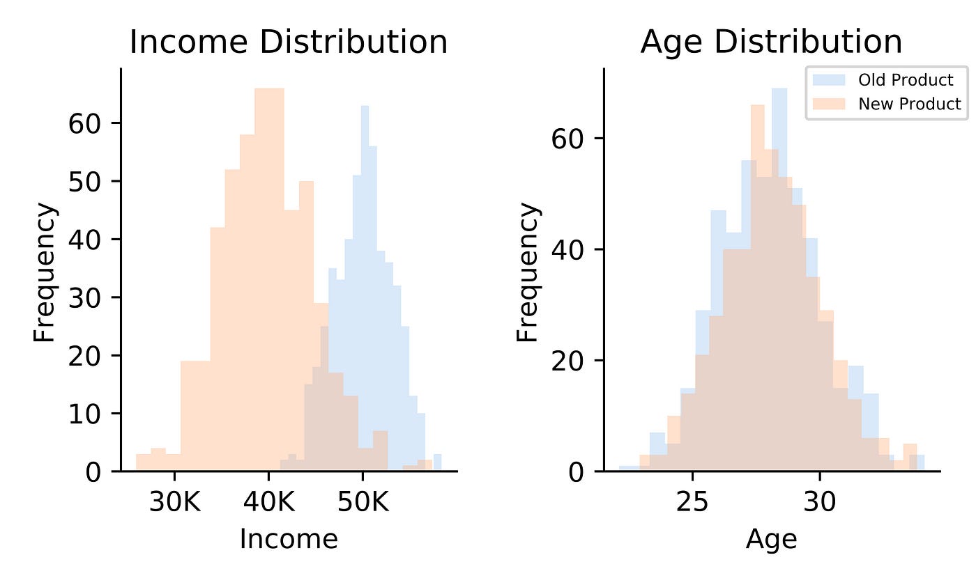
To deliver a story, we can analyze the demographic data and respond the post-obit questions:
- are the 2 groups of customers like in terms of historic period?
- are the two groups of customers making similar incomes?
Answering these questions entails comparison two sample distributions, which tin can be done using the discrete KS test. As a event of this exam, we will detect out whether we should proceed or discontinue the sometime product line.
What is the idea behind the discrete KS test?
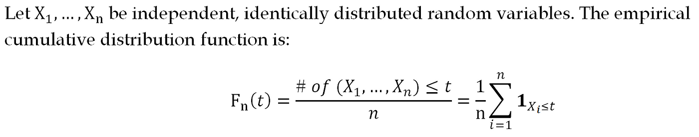
The thought behind the KS exam is simple: if two samples vest to each other, their empirical cumulative distribution functions (ECDFs) must be quite similar. This suggests that we can evaluate their similarity by measuring the differences between the ECDFs.
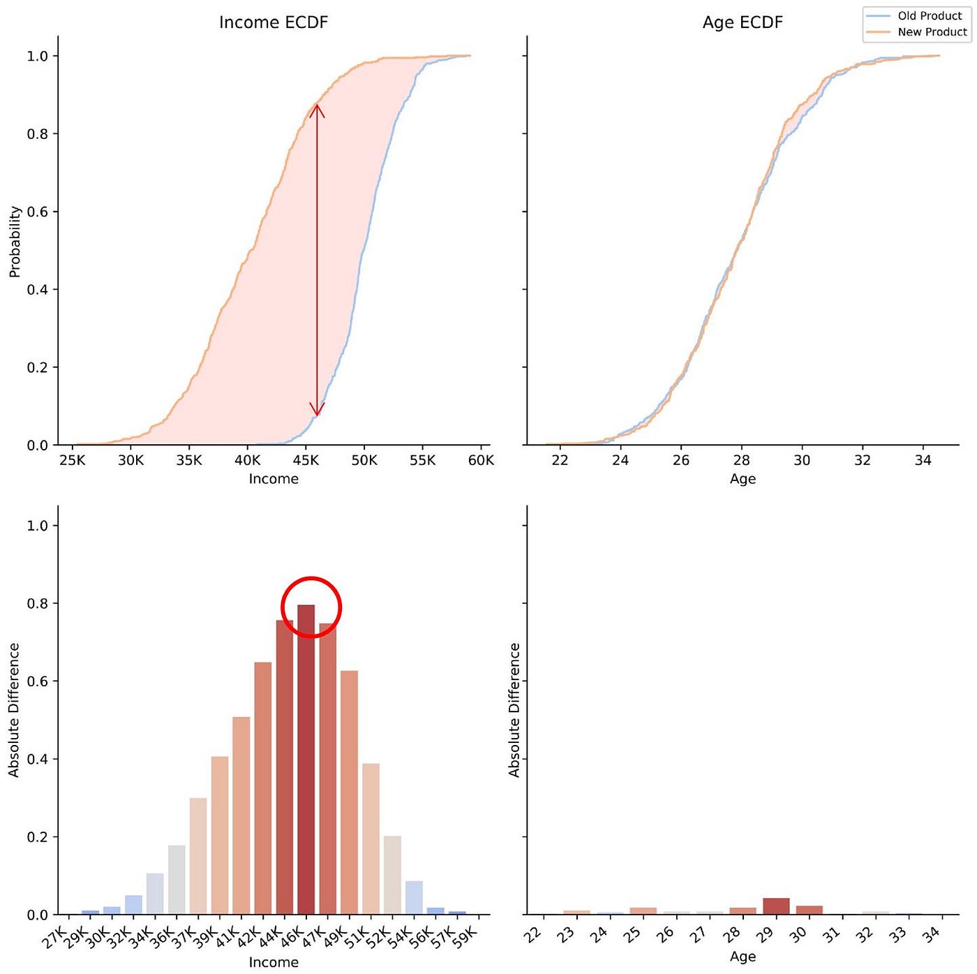
To achieve this, the KS test finds the maximum distance between the ECDFs. More chiefly, the test requires evaluating whether the distance is large enough to merits that the two samples practise not belong to each other.
In the diagram below, the maximum distance between the income ECDFs is indicated past the red pointer. The scarlet pointer corresponds to the KS test statistic and is shown in the crimson circumvolve.
In practice, the detached version of the KS test is often appropriate because of rounding. Although variables such as time and toll are theoretically continuous, these are oftentimes considered discrete variables due to rounding, which gives the states a finite fix of possible values. The continuous version of the KS test can however be used although it volition pb to a more conservative result (i.eastward. if the rejection level is 5%, the actual level will exist less than 5%).
How practise we apply the discrete KS test?
The post-obit is a procedure to conduct the discrete KS test for two samples:
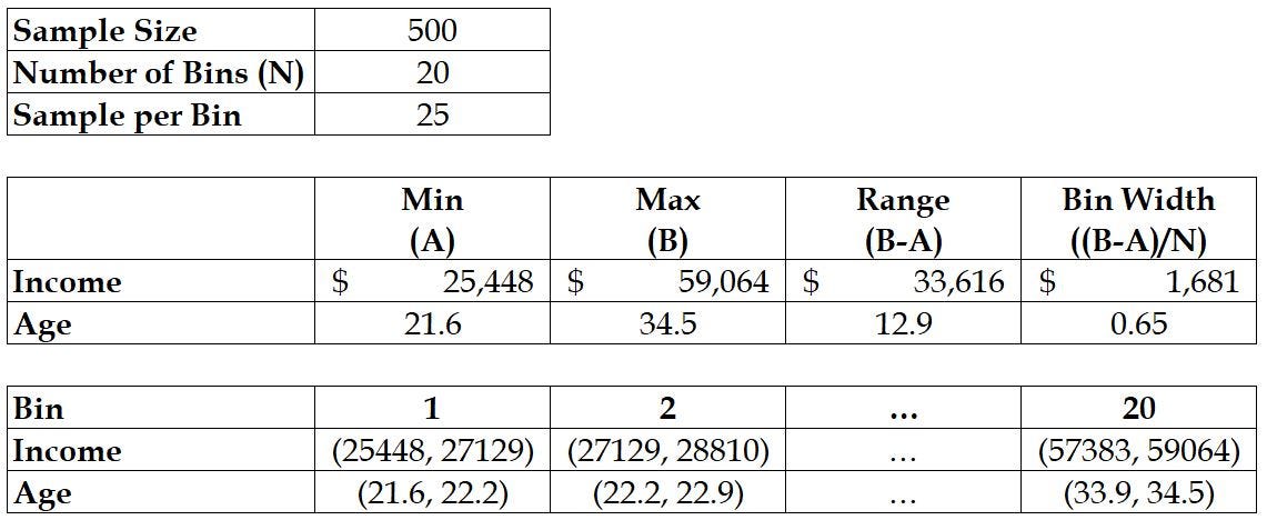
Stage one: Binning the range
- Find the min and max of the combined sample to define our range.
- Bin the range such that there are at least 10 samples per bin:
east.k. for a sample size of 500, we tin expect 25 samples per bin by choosing 20 buckets.
Stage two: Counting the bin frequencies
- With the set of bins from Phase 1, use the ECDF formula from the previous section to compute the frequencies of all bins for each sample.
Stage 3: Calculating the maximum distance
- For each bin, compute the difference in frequencies between the two samples.
- The KS examination statistic is equal to the largest difference in frequencies amidst all bins.
How practise we make sense of the KS test statistic?
To find out whether we tin refuse the null hypothesis or not, we have to derive a KS examination statistics distribution using statistical techniques.
1. Sample distribution vs. theoretical distribution
When we compare a sample with a theoretical distribution, nosotros can use a Monte Carlo simulation to create a test statistics distribution.
For case, if we want to test whether a p-value distribution is uniformly distributed (i.e. p-value uniformity test) or not, nosotros can simulate uniform random variables and compute the KS test statistic. Past repeating this process 1000 times, we will have 1000 KS test statistics, which gives us the KS test statistic distribution below.

By inserting the KS test statistic for the actual sample (i.eastward. the ruby-red line), nosotros can come across that the actual KS examination statistic is contained inside the distribution. This means that there is no strong evidence confronting the goose egg hypothesis that the p-value sample follows a uniform distribution.
Furthermore, the dark-green line, which represents the KS exam statistics from a simulation using m normal random variables, is outside the distribution. This manifests the contrast betwixt a uniform and normal distribution.
2. Sample distribution vs. some other sample distribution
In our before example with historic period and income distributions, we compared a sample distribution to another sample distribution instead of a theoretical distribution. In this case, we demand to apply resampling techniques such every bit permutation tests or bootstrapping to derive a KS exam statistic distribution.
In this section, we volition comport a permutation test, which involves combining both samples to randomly create new sets of two samples. With each new set, nosotros volition compute the KS exam statistic and combine all of them to generate the KS test statistic distribution.
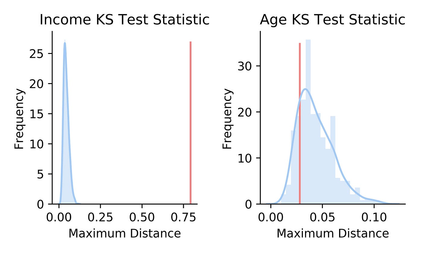
As expected, the KS test statistic for the actual income samples is far away from the distribution. This suggests we tin reject the naught hypothesis that states the income samples are identical (i.east. p-value is cypher). In dissimilarity, the KS test statistic of the actual age samples is located within its KS exam statistic distribution. Hence, nosotros cannot decline the zip hypothesis that states the age samples are identical.
What nosotros have learned
Equally a consequence of our findings, we can conclude that the new and old product may be targeting a like age grouping, but different income groups. This tells united states of america that we should not discontinue the onetime product and must discover an optimal residual between the two products.
Bated from the KS test, there are alternatives such as the chi-foursquare and Anderson-Darling (Ad) tests, which can be establish in [ii]. In comparison to the KS test, which puts all emphasis on the bin with the largest divergence, these alternatives allocate weights among all bins. The chi-foursquare examination allocates weights based on the expected frequencies of the bins while the AD test puts more accent on the tail.
I would similar to encourage the readers to utilize the discrete KS exam or explore other alternatives as office of their analytic routines. Not but practise these tests help us understand data inside out, but they also are elementary to implement. There is an R bundle available here. Have fun and make the all-time of it!
Sources
[1] Elmore, Chiliad. L. (2005). Alternatives to the Chi-Square Test for Evaluating Rank Histograms from Ensemble Forecasts. Conditions and Forecasting, 20(5), 789–795. doi: x.1175/waf884.1
[2] Steele, Chiliad., & Chaseling, J. (2006). Goodness-of-Fit Tests Powers of Discrete Goodness-of-Fit Exam Statistics for a Uniform Zip Against a Selection of Alternative Distributions.
Source: https://towardsdatascience.com/how-to-compare-two-distributions-in-practice-8c676904a285
Postar um comentário for "what does it mean for two distributions to be identical"